
Excel becomes truly powerful when you know how to pull the right data at the right time. One such function that quietly saves hours of manual work is the HLOOKUP formula in Excel. It is especially useful when your data is arranged horizontally instead of vertically. Many users ignore it, but when used correctly, it can simplify reporting, analysis, and everyday office tasks.
What Is the HLOOKUP Formula in Excel and Why It Matters
Understanding the basic concept of HLOOKUP
The HLOOKUP function in Excel is designed to search for a value in the top row of a table and return a related value from a specified row below it. The “H” in HLOOKUP stands for Horizontal, which means the data runs left to right.
For example, if months are placed across the top row and sales figures are listed below, HLOOKUP helps you fetch sales for a specific month instantly. This is useful when working with dashboards, performance sheets, or summary tables.
When should you use HLOOKUP instead of VLOOKUP
However, not all data fits a vertical format. In addition, many legacy Excel sheets store headers in rows, not columns. In such cases, HLOOKUP becomes the natural choice.
Use HLOOKUP when:
-
Headers are in the first row
-
Data extends horizontally
-
You want to avoid restructuring existing sheets
As a result, HLOOKUP saves time and reduces errors caused by manual searching.
Real-life example where HLOOKUP helps
Imagine a school marksheet where subjects are listed in the top row and student scores are below. Instead of scrolling, HLOOKUP can quickly pull the required marks. Therefore, it works well for reports that repeat the same lookup logic daily.
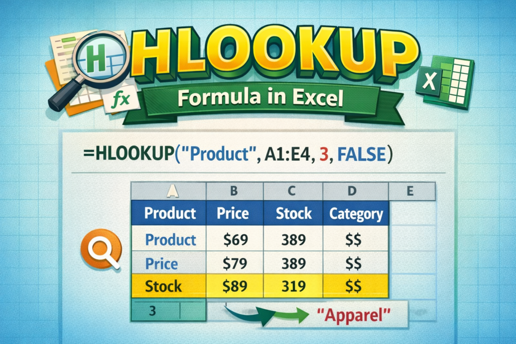
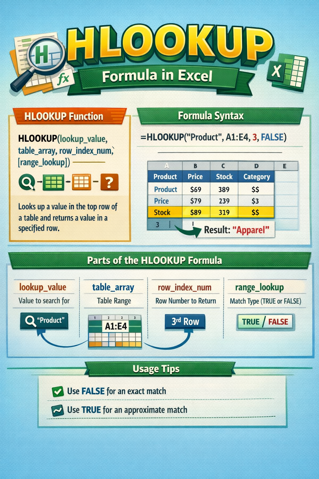
HLOOKUP Formula Syntax Explained with Easy Examples
Basic syntax of the HLOOKUP function
The syntax of the HLOOKUP formula in Excel looks like this:
HLOOKUP(lookup_value, table_array, row_index_num, [range_lookup])
Although it may look technical, each part has a simple role.
-
lookup_value: The value you want to find
-
table_array: The data range
-
row_index_num: The row number to return data from
-
range_lookup: Exact or approximate match
Moreover, once you understand these parts, writing the formula becomes intuitive.
Simple HLOOKUP example for beginners
Suppose cell A1 contains the month “March”. Your data is in A1:F4, with months in row 1 and sales in row 2.
Formula:
HLOOKUP(A1, A1:F4, 2, FALSE)
As a result, Excel returns March sales without scanning the sheet manually.
Exact match vs approximate match
If you use FALSE, Excel looks for an exact match. This is ideal for text values like names or months. On the other hand, TRUE is useful for approximate matches, such as tax slabs or commission rates.
Therefore, choosing the correct option avoids incorrect results.
Practical Use Cases of HLOOKUP in Excel Sheets
Using HLOOKUP for monthly sales reports
Many businesses track months horizontally. HLOOKUP helps retrieve revenue, expenses, or profit figures instantly. In addition, it keeps reports clean and readable.
Instead of copying formulas repeatedly, one HLOOKUP can power multiple cells. This reduces human error and improves productivity.
Student results and exam score analysis
Teachers often store subjects across rows. HLOOKUP allows them to fetch marks for a particular subject quickly. Moreover, it supports dynamic analysis when combined with dropdown lists.
This approach also makes result sheets more interactive and professional.
Inventory and product comparison tables
For example, product features listed across the top row can be compared easily using HLOOKUP. As a result, decision-making becomes faster, especially in procurement or pricing analysis.
Therefore, HLOOKUP fits well into daily office workflows.
Common Errors in HLOOKUP and How to Fix Them
#N/A error in HLOOKUP
One of the most common issues is the #N/A error. This usually appears when Excel cannot find the lookup value. However, the problem is often simple.
Check if:
-
The lookup value exists in the top row
-
Extra spaces are present
-
Exact match is required but FALSE is missing
Moreover, using TRIM can solve spacing issues.
Incorrect row index number
Another frequent mistake is selecting the wrong row index number. Remember, Excel counts rows from the top of the table array, not the worksheet.
For example, if your return value is in the third row of the table array, the row index should be 3. Otherwise, Excel returns incorrect data.
Making HLOOKUP safer with IFERROR
To avoid ugly error messages, wrap your formula with IFERROR.
Example:
IFERROR(HLOOKUP(A1, A1:F4, 2, FALSE), “Not Found”)
As a result, your sheet looks cleaner and more professional.
HLOOKUP vs VLOOKUP vs XLOOKUP: Which One Should You Use
Key differences between HLOOKUP and VLOOKUP
The main difference lies in data direction. HLOOKUP works horizontally, while VLOOKUP works vertically. However, both have similar limitations.
For instance, both functions rely on fixed index numbers, which can break formulas when rows or columns change.
Why XLOOKUP is gaining popularity
XLOOKUP is more flexible and modern. It works in any direction and does not require index numbers. However, it is only available in newer Excel versions.
Still, many offices use older Excel versions. Therefore, knowing HLOOKUP remains valuable.
When HLOOKUP still makes sense
If your data is already structured horizontally and you use older Excel versions, HLOOKUP is still the right tool. Moreover, it is easier to understand for beginners.
As a result, mastering HLOOKUP builds a strong Excel foundation.
Frequently Asked Questions About HLOOKUP Formula in Excel
What is the HLOOKUP formula in Excel used for?
The HLOOKUP formula in Excel is used to search for a value in the top row of a table and return a corresponding value from a row below. It is ideal for horizontally arranged data like months, subjects, or product features.
How do I use HLOOKUP with exact match?
To use HLOOKUP with exact match, set the range_lookup argument to FALSE. This ensures Excel returns a value only when it finds an exact match in the top row, which is useful for text-based lookups.
Why is my HLOOKUP returning #N/A?
HLOOKUP returns #N/A when the lookup value is not found in the first row of the selected table. This can happen due to spelling differences, extra spaces, or incorrect range selection.
Can HLOOKUP return text values?
Yes, HLOOKUP can return both text and numeric values. As long as the return row contains text data, Excel will display it correctly without additional formatting.
Is HLOOKUP case-sensitive?
No, HLOOKUP is not case-sensitive. It treats “January” and “january” as the same value. However, extra spaces can still cause errors.
What is the alternative to HLOOKUP in modern Excel?
XLOOKUP is the best alternative in modern Excel versions. It is more flexible and easier to maintain. However, HLOOKUP is still widely used in older Excel files.
Can I combine HLOOKUP with other formulas?
Yes, HLOOKUP works well with IF, IFERROR, MATCH, and dropdown lists. This combination allows you to build dynamic and user-friendly Excel dashboards.
Final Thoughts on Using HLOOKUP Effectively
The HLOOKUP formula in Excel may not be as popular as newer functions, but it still plays an important role in real-world spreadsheets. When data is arranged horizontally, it offers a clean and reliable solution. Moreover, understanding HLOOKUP improves your overall Excel confidence.
If you regularly work with reports, marksheets, or comparison tables, mastering this function can save time and reduce errors. Practice it with small datasets, and soon it will feel natural. Over time, this simple formula can quietly become one of your most trusted Excel tools.